Encoding a magic state with beyond break-even fidelity

To run large-scale algorithms on a quantum computer, error-correcting codes must be able to perform a fundamental set of operations, called logic gates, while isolating the encoded information from noise1,2,3,4,5,6,7,8. We can complete a universal set of logic gates by producing special resources called magic states9,10,11. It is therefore important to produce high-fidelity magic states to conduct algorithms while introducing a minimal amount of noise to the computation. Here we propose and implement a scheme to prepare a magic state on a superconducting qubit array using error correction. We find that our scheme produces better magic states than those that can be prepared using the individual qubits of the device. This demonstrates a fundamental principle of fault-tolerant quantum computing12, namely, that we can use error correction to improve the quality of logic gates with noisy qubits. Moreover, we show that the yield of magic states can be increased using adaptive circuits, in which the circuit elements are changed depending on the outcome of mid-circuit measurements. This demonstrates an essential capability needed for many error-correction subroutines. We believe that our prototype will be invaluable in the future as it can reduce the number of physical qubits needed to produce high-fidelity magic states in large-scale quantum-computing architectures.
Error mitigation extends the computational reach of a noisy quantum processor
Article 27 March 2019
Removing leakage-induced correlated errors in superconducting quantum error correction
Article Open access
19 March 2021
Protecting a bosonic qubit with autonomous quantum error correction
Article 10 February 2021
Main
We distil magic states to complete a universal set of fault-tolerant logic gates that is needed for large-scale quantum computing with low-density parity-check code architectures13,14,15,16,17,18. High-fidelity magic states are produced9,10,11 by processing noisy input magic states with fault-tolerant distillation circuits; experimental progress in preparing input magic states using trapped-ion architectures is described in refs. 3,7. It is expected that a considerable number of the qubits of a quantum computer will be occupied performing magic-state distillation schemes and, as such, it is valuable to find ways of reducing its cost. One way to reduce the cost is to improve the fidelity of input states11,19,20,21,22,23,24,25,26, such that magic states can be distilled with less resource-intensive circuits.
Here we propose and implement an error-suppressed encoding circuit to prepare a state that is input to magic-state distillation using a heavy-hexagonal lattice of superconducting qubits4,5,27. Our circuit prepares an input magic state, which we call a CZ state, encoded on a four-qubit error-detecting code. We explain how our encoded magic state can be used in large-scale quantum-computing architectures11,28 in the section ‘Using CZ states in large-scale quantum-computing architectures’. Our circuit is capable of detecting any single error during state preparation, as such, the infidelity of the encoded state is suppressed as �(ε2)
, where ε is the probability that a circuit element experiences an error. By contrast, a standard encoding circuit prepares an input state with infidelity �(ε)
. Furthermore, we can improve the yield of the prepared magic states with the error-suppressed circuit using adaptive circuits that are conditioned in real time on the outcomes of mid-circuit measurements. We propose several tomographical experiments to interrogate the preparation of the magic state, including a complete set of fault-tolerant projective logical Pauli measurements that can also tolerate the occurrence of a single error during readout.
Magic-state preparation and logical tomography
We prepare the CZ state as follows:
|��⟩≡|00⟩+|01⟩+|10⟩3,
encoded on a distance-2 error-detecting code, in which the distinct bit strings label orthogonal computational basis states over two qubits. We can achieve the CZ state by, first, preparing the |++⟩=∑�,�=0,1|��⟩/2
state and, then, projecting it onto the CZ = +1 eigenspace of the controlled-phase (CZ) operator CZ = diag(1, 1, 1, −1), that is, |��⟩∝Π+|++⟩
with the projector 𝟙
Π+=(𝟙+��)/2
. We can perform both these operations with the four-qubit code. Specifically, it has a fault-tolerant preparation of the |++⟩ state and, as we will show, we can make a fault-tolerant measurement of the logical CZ operator to prepare an encoded CZ state.
Encoded states of the four-qubit code lie in the common +1 eigenvalue eigenspace of its stabilizer operators SX = X ⊗ X ⊗ X ⊗ X, SZ = Z ⊗ Z ⊗ Z ⊗ Z and SY = SZSX, where X and Z are the standard Pauli matrices. The four-qubit code encodes two logical qubits that are readily prepared in a logical |+¯+¯⟩
state by initializing four data qubits in the superposition state, |+⟩ ∝ |0⟩ + |1⟩, and measuring SZ. We note that we use bars to indicate we are describing states and operations in the logical subspace. We prepare the state with SZ = +1 using either post-selection or, alternatively, an adaptive Pauli-X rotation on a single-qubit given a random −1 outcome from the SZ measurement.
The four-qubit code has a transversal implementation of the CZ gate on its encoded subspace, ��¯≃�⊗�†⊗�†⊗�
, where �=diag(1,�)
. We can measure this operator as follows. We note that conjugating SX with the unitary rotation �~=�⊗�†⊗�†⊗�
, where �=diag(1,�)
, gives the Hermitian operator:
�¯≡�~���~†∝��¯��.
(1)
Given that we prepare the code with SX = +1, measuring �¯
effectively gives a reading of ��¯
.
It is essential to our scheme that we reach the SZ = +1 eigenspace. This is because of the non-trivial commutation relations of �¯
with the stabilizer operators of the code29,30; [��,�¯]=(1−��)���¯
. This commutator shows that �¯
only commutes with SX in the SZ = +1 subspace. If SZ = −1, we can check that �¯
and SX anti-commute, and are therefore incompatible observables in this subspace.
We can perform all of the aforementioned measurements, SX, �¯
and SZ, on the heavy-hexagon lattice geometry27. Figure 1 shows one such setup. The circuit is fault-tolerant in the sense that a Pauli error introduced by a circuit element, on the support of the circuit element, is always detected by a flag qubit or a stabilizer measurement. The verification of this is detailed in the section ‘Analysis in terms of single-gate errors’.
Fig. 1: A fault-tolerant circuit to make parity measurements.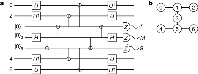 a, A circuit that measures SX, SZ and �¯
using flag qubits on the heavy-hexagonal lattice architecture. b, The four-qubit code is encoded on qubits with even indices and the other qubits are used to make the fault-tolerant parity measurement. The circuit measures SX by setting 𝟙
�=𝟙
and SZ by setting U = H, where H is the Hadamard gate. The circuit measures �¯
if we set U = T. The measurement outcome M gives the reading of the parity measurement. Essential to the fault-tolerant procedure are flag fault-tolerant readout circuits4,5,27,51 that identify errors that occur during the parity measurement. Outcomes f and g are flag qubit readings that indicate that the circuit may have introduced a logical error to the data qubits.
We, therefore, present a sequence of measurements that prepare the input magic state and, in tandem, identify a single error that may have occurred during the preparation procedure. Figure 2 shows the sequence and describes its function. As we can detect a single error, we expect the infidelity of the output state to be �(ε2)
. We compare our error-suppressed magic-state preparation scheme to a standard scheme for encoding a two-qubit magic state, as well as a circuit that prepares the magic state on two physical qubits. Both of these schemes are described in the section ‘Standard magic-state preparation circuits’.
Fig. 2: Fault-tolerant schemes for magic-state preparation and logical tomography.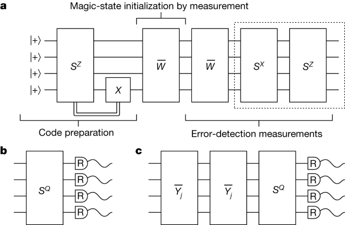 a, Preparation of a CZ state on a four-qubit code in three steps. In the code-preparation step, the four-qubit code is prepared in the logical |+¯+¯⟩
state by measuring |+⟩⊗4
with the SZ operator. We can use adaptive circuits or post-selection to correct for SZ = −1 outcomes. In the magic-state initialization step, we measure the �¯
operator and post-select on the +1 outcome. In the final error-detection step, we identify the errors that may have occurred during preparation. We measure �¯
a second time to identify if a measurement error occurred during the magic-state initialization step. We finally measure SX and SZ a second time to identify Pauli errors that may have occurred, and to determine if the initial SZ measurement gave a readout error. b,c, We replace the parity measurements in the dashed box of a with circuits b and c to make logical tomographic measurements and, at the same time, infer a complete set of stabilizer data for error detection. For example, if we set SQ = SX and measure qubits in the R = Z basis, we infer the value of SZ, as in a, and we also obtain readings of the logical �¯1
, �¯2
and �¯1�¯2
. Likewise, we can set SQ = SZ with either R = X to infer SX as well as logical Pauli operators �1¯
, �2¯
and �1¯�2¯
, or R = Y to infer SY as well as logical Pauli operators �1¯�2¯
, �1¯�2¯
and �1¯�2¯
. In c, we include a �¯�
measurement for logical qubit j = 1, 2 to measure logical operators of the form �¯�
, �¯���¯
and �¯���¯
with k ≠ j and k = 1, 2, where we take an appropriate choice of R. The �¯�
operator is measured twice to identify the occurrence of measurement errors. Operators �¯�
are supported on three of the data qubits and can therefore be read out with an appropriate modification of the circuit shown in Fig. 1.
We verify our state-preparation schemes by performing two variants of quantum-state tomography to reconstruct the logical state. The first method uses fault-tolerant circuits that directly measure the logical operators; we refer to this tomographical method as ‘logical tomography’. For the second method, which we refer to as ‘physical tomography’, we perform standard state tomography on the full state of the four data qubits of the system and then project the reconstructed state onto the logical subspace. Logical tomography with the four-qubit code is shown in Fig. 2b,c. All of our logical tomography circuits can tolerate a single error at the readout stage, by repeating the measurement of logical operators and by comparing measurement outcomes to earlier readings of stabilizer measurements.
Logical tomography is more efficient than physical tomography because we are directly measuring and reconstructing the encoded logical state, rather than the physical state. In the case of the four-qubit code, this requires only 7 distinct circuits, whereas physical tomography requires 81 different measurement circuits.
Experimental results
We performed our experiments using the first-generation real-time control system architecture of IBM Quantum deployed on ibm_peekskill; one of the IBM Quantum Falcon Processors (https://quantum.ibm.com/). Device characterization can be found in the section ‘Device overview’. The control system architectures give access to dynamic circuit operations, such as real-time adaptive circuit operations that depend on the outcomes of mid-circuit measurements, that is, feedforward (see section ‘Real-time feedforward control of qubits’).
Our results are shown in Fig. 3, in which we present state infidelities for various state-preparation schemes calculated using both logical tomography and physical tomography. For results provided in the main text, we model the reconstructed state assuming that the readout is conducted with projective measurements. We also present an alternative analysis in the section ‘State tomography with readout error mitigation using noisy positive-operator-valued measurements’, in which we combine the readout error characterization with tomographic reconstruction using noisy positive-operator-valued measurements.
Fig. 3: Infidelities measured in magic-state preparation experiments.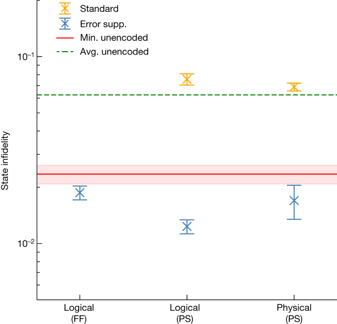 State infidelity for error-suppressed (error supp.) and standard schemes are shown in blue and orange, respectively. On the x-axis, a state is reconstructed with either logical or physical tomography. The correction for the initial SZ measurement in Fig. 2a is implemented using either real-time feedforward (FF) or post-selection (PS). For the physical data points, the state from physical tomography is projected onto the logical subspace before computing the infidelity by fitting to ideal projectors. Error bars represent 1σ from bootstrapping. For all tomographic methods, the error-suppressed scheme achieves a lower state infidelity compared with the standard scheme. The unencoded magic state prepared directly on two physical qubits gives an average (avg.) infidelity across 28 qubit pairs as approximately 6.2 × 10⁻² (green dashed line) using 18 repetitions over a 24-h period with 105 shots per circuit. Of these, the best-performing pair yields a minimum (min.) infidelity of (2.354 ± 0.271) × 10−2 (red solid line) found over all repetitions for all qubit pairs. In all cases, the error-suppressed scheme exceeds the fidelity of the best two-qubit unencoded magic state.
To accommodate drift in device parameters over the data collection period, a complete set of tomography circuits was interleaved and submitted in batches of about 104 shots until a total of about 106 shots were collected over several days. The resulting counts database is uniformly sampled with a replacement for 10 bootstrap trials with a batch size limited to 20% of the total database before post-selection. The standard deviation, σ, of these bootstrapped trials is plotted as an error bar in all data figures.
The tomographic fitting was done using positive semi-definite constrained weight-least-squares convex optimization using the Qiskit Experiments tomography module31. For logical tomography, the fitting weights were set proportional to the inverse of the standard errors for each logical Pauli expectation value estimate. These weights accommodate the different logical yield rates for each logical Pauli measurement. The logical yield for each basis measurement is shown in Fig. 4 and discussed in more detail below.
Fig. 4: Magic-state yield for feedforward versus post-selection.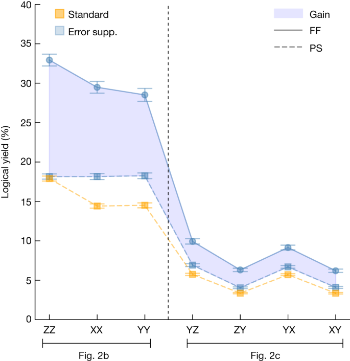 Yield is calculated for logical tomography circuits shown in Fig. 2b,c for the error-suppressed (error supp.) scheme with feedforward (blue circles) versus post-selection (blue squares); a standard scheme is shown for reference (orange squares). All rates use datasets reported in Fig. 3 where error bars represent 1σ from bootstrapping. The shaded area of the graph shows the increase in yield for the error-suppressed scheme using feedforward (FF) compared with the post-selection (PS) scheme or the standard scheme. The optimal acceptance rate assuming no noise is 75% for the feedforward scheme, 37.5% for the post-selection scheme and 25% for the standard scheme. The observed acceptance rates are because of the additional detection of errors. We estimate the yield in the presence of noise in the section ‘Estimates for magic-state yield’. We observe a stark difference in yields between experiments conducted with the logical tomography circuit shown in Fig. 2b,c, shown to the left and right of the dashed line, respectively. We can attribute this to the depth of the logical tomography circuit, in which deeper circuits, such as those shown in Fig. 2c, are more likely to introduce detectable errors. This is discussed in the section ‘Estimates for magic-state yield’.
We first compare the state-preparation scheme using dynamic circuits with the same preparation scheme executed with static circuits and post-selection. This comparison is conducted using logical tomography. These are the left and middle data points shown in blue in Fig. 3. We find that the infidelities are commensurate in these two experiments. Using dynamic circuits with feedforward operations, we encode a two-qubit error-suppressed input magic state with a logical infidelity (1.87 ± 0.16) × 10−2. In the post-selection experiment, we obtain an infidelity of (1.23 ± 0.11) × 10−2. The feedforward operations in our experiment can introduce idling periods, of the order of hundreds of nanoseconds, during which additional errors can accumulate. To leading order we attribute the difference in fidelity between these preparation schemes to errors that occur while the control system is occupied performing the dynamical feedforward operation. In return for this loss in fidelity, we find that the use of dynamical circuits significantly increases the yield of magic states (Fig. 4).
We can analyse the commonly occurring errors in fault-tolerant circuits using syndrome outcomes to infer the events that are likely to have caused them32. This is done using the method detailed in the section ‘Analysis in terms of single-gate errors’ using the results of the error-suppressed scheme without any post-selection. Assuming an uncorrelated error model, we find that the average probability per single-error event is 0.19% with a standard deviation of 0.11%. The single most-likely error event occurs with probability 1.2%. This event corresponds to an error occurring during the X stabilizer measurement that spreads to and is detected by a flag qubit. Similar errors in other stabilizer measurements show the probability increasing from 0.35% for the initial Z measurement to 0.41% and 0.45% for the two �¯
measurements. This suggests that, rather than being caused by Pauli errors, these results might be caused by other effects such as an accumulation of leakage on the flag qubits.
We verify the performance of our logical tomography procedure by comparing our results with the infidelity obtained using physical tomography for the magic-state preparation procedure, in which we obtain the SZ = +1 eigenspace with post-selection. The fitter weights in this case are the standard Gaussian weights based on the observed frequencies of each projective measurement outcome of each basis element. In physical tomography, the yield after post-selection is constant in all 81 measurement bases. We find an acceptance rate of 14.9 ± 0.1% for the error-suppressed scheme using physical tomography, in which the standard deviation represents variation over 81 physical Pauli directions.
To compare the infidelity obtained with physical tomography even-handedly with that obtained using logical tomography, we reconstruct the logical subspace from the density matrix obtained from physical tomography on the data qubits of the code, ρphys. The logical subspace is obtained by projecting ρphys onto the logical subspace33,34. We obtain the elements of the density matrix of the logical subspace ρ using the equation
���,��=⟨�¯�¯|�phys|�¯�¯⟩��,
(2)
where k, l, m, n = 0, 1 specify orthogonal vectors in the logical subspace and ��=∑�,�⟨�¯�¯|�|�¯�¯⟩
is the probability that the state we prepare is in the logical subspace. Using this method, we obtain the projected logical infidelity for the error-suppressed procedure as (1.70 ± 0.35) × 10−2 with the probability of finding ρphys in the logical subspace PL = 0.898 ± 0.008. An average post-selection acceptance rate over all physical Pauli directions is found to be 14.9 ± 0.1%. This projected logical infidelity is shown as the rightmost blue data point in Fig. 3 to be compared with the central blue data point. This comparison demonstrates the consistency between logical tomography and physical tomography. For reference, raw state fidelities from physical tomography before logical projection are reported in the section ‘State tomography with readout error mitigation using noisy positive-operator-valued measurements’.
We compare our error-suppressed magic-state preparation procedure with a standard static circuit that encodes a physical copy of the magic state into the four-qubit code. We show infidelity data points for the standard scheme in Fig. 3 with orange markers. Our experiments consistently demonstrate that our error-suppressed encoding scheme has an infidelity at least four times smaller than a standard scheme to encode magic states. We show yields using different logical tomography experiments for the standard preparation scheme with orange markers in Fig. 4. In the case of physical tomography, the encoded state on the four data qubits has a post-selection acceptance rate of 20.9 ± 0.1%, and the reconstructed density matrix is found in the code space with probability PL = 0.789 ± 0.004.
Finally, we compare our error-suppressed preparation procedure with a state-preparation experiment performed using physical qubits. We mark the lowest infidelity obtained over all of the adjacent pairs of physical qubits on the 27 qubit device, (2.4 ± 0.3) × 10−2, with a red line in Fig. 3. Remarkably, all fidelities for all of our error-suppressed magic-state preparation schemes exceed the fidelity of a simple experiment to prepare the CZ state with physical qubits.
Discussion
We have presented a scheme that encodes an input magic state with a fidelity higher than we can achieve with any pair of physical qubits on the same device using basic entangling operations. This improvement in fidelity, which is beyond the break-even point set by basic physical qubit operations, can be attributed to quantum error correction that suppresses the noise that accumulates during state preparation.
The yield of magic states benefited from the use of dynamic circuits in which mid-circuit measurements condition gate operations in real time. Remarkably, we find that the operation is sufficiently rapid that its execution came at only a small cost in output state fidelity on the superconducting device. These dynamic circuits are essential to future quantum-computing architectures as they will be needed, for example, to perform magic-state distillation circuits9,10,11 and gate teleportation35,36, as well as many other measurement-based methods13,17,18,19,37,38,39,40,41,42,43,44,45,46,47,48 that have been proposed to complete a universal set of logic gates.
We have shown that experimental progress has reached a point at which we can make prototype gadgets that can affect the resource cost of large-scale quantum computers. In the Methods, we explain how our prototype can be used together with magic-state distillation. It will be interesting to continue to design, develop and test new gadgets with real hardware that will improve the performance of the key subroutines needed for fault-tolerant quantum computing. Further developments in the theory of pieceable fault tolerance44 might show us ways of producing better magic states with small devices. Error-suppressed magic states could improve the time cost of recent proposals49,50 for error-corrected circuits that are supplemented by error-mitigation techniques to complete non-Clifford operations. Ultimately, experimental progress that we make to this end in the near term can benefit large-scale quantum-computing architectures.
Methods
Using CZ states in large-scale quantum-computing architectures
Magic states are distilled to complete a universal set of fault-tolerant logic gates (see Extended Data Fig. 1 for an overview of the details of a generic magic-state distillation protocol). In any such protocol, input magic states with some inherent error are encoded on quantum error-correcting codes. The encoded magic states are then used in distillation circuits to produce better magic states with higher fidelity. We can use magic states with near-perfect fidelity to perform fault-tolerant logic gates.
We choose different magic-state distillation protocols depending on the magic states we prepare. In the next section, we review details on how we can use CZ states in large-scale fault-tolerant quantum computing. Specifically, we can convert CZ states into Toffoli states using Pauli measurements and Clifford operations28, such that we can adopt well-known magic-state distillation protocols for further rounds of distillation11. This conversion technique is probabilistic, as it depends on obtaining the correct outcome from a Pauli measurement. In addition to these results, we show how we can recover a CZ state from the output state, assuming we get the incorrect outcome of the Pauli measurement, thereby conserving the available resource states.
We also provide some examples of how we can inject small codes into larger codes in the section ‘Injecting small codes into larger codes’, as it will be required to take the encoded state we prepared in the main text and use it in subsequent rounds of magic-state distillation. Specifically, we show how to take distance-2 codes and encode their state on the surface code, the heavy-hex code and the colour code with a higher distance. Notably, the heavy-hex code is readily implemented on the heavy-hex lattice geometry on which we conducted the experiment. For each of these injection schemes, we argue that we can detect any single error that may occur. This is important to maintain the error suppression obtained when preparing the CZ state.
In the case of the colour-code state-injection protocol, we inject the error-detecting code described in the main text directly into the larger code. In the case of the surface code and heavy-hex code, however, we inject a related code, that we call the [[4, 1, 2]] code. To complete these injection protocols, we need to take the CZ state prepared on the error-detecting code and copy its logical state onto two copies of the [[4, 1, 2]] code. We give a fault-tolerant procedure for this transformation in the section ‘Encoding the CZ state on two [[4, 1, 2]] codes using the heavy-hex lattice geometry’.
Magic-state distillation with the CZ state
Although magic-state distillation for the CZ state has not been well-studied in the literature, it is known that two copies of the state can be probabilistically converted into a Toffoli state using Pauli measurements and Clifford operations28. Given there are known methods for distilling Toffoli states11, let us review how the Toffoli state is produced from the copies of the CZ state. In the following sections, we show how to inject the CZ state into larger quantum error-correcting codes that are capable of performing fault-tolerant Clifford operations17,18,45 to complete these circuits.
The Toffoli state is defined as follows:
|TOF⟩∝∑�,�|�⟩|�⟩|��⟩=|000⟩+|010⟩+|100⟩+|111⟩,
(3)
where we sum over the bitwise values j, k = 0, 1.
Given two copies of the CZ state, |��⟩1,2|��⟩3,4
, if we project qubits 2 and 3 onto the Z2Z3 = −1 eigenspace, then we obtain the intermediate state
|�⟩=(|0010⟩+|1010⟩+|0100⟩+|0101⟩)/2.
(4)
We then obtain |1⟩|TOF⟩
with the following unitary circuit
|1⟩|TOF⟩=��4,3��3,1��2,1��1,3|�⟩,
(5)
where indices C and T of the controlled-not gate CXC,T denote the control and target qubit, respectively.
We obtain the −1 outcome by measuring Z2Z3 of state |��⟩|��⟩
with probability 4/9. Beyond the work in ref. 28, we find that we can recover a single copy of the CZ state given the Z2Z3 = +1 outcome at this step, thereby saving magic resource states. In the event that we obtain this measurement outcome, we produce the state
|�⟩=|0000⟩+|0001⟩+|1000⟩+|1001⟩+|0110⟩.
(6)
Applying the unitary operation ��2,3��2,4|�⟩
and obtaining the two-qubit parity measurement outcome Z3Z4 = −1, we obtain the state |��⟩|01⟩
. We obtain this state with probability 3/5, assuming we obtained the Z2Z3 = +1 outcome previously.