The Math Behind K-Nearest NeighborsWhy is K-Nearest Neighbors one of the most popular machine-learn

Image generated by DALL-E
K-Nearest Neighbors is one of the most popular machine-learning algorithms out there. Its simplicity, versatility, and adaptability make it a common choice. But, why is it so popular? Why does it perform so well? This article peels back the layers of KNN, revealing how it works and why it’s a favored tool for many data scientists. We’ll look at its applications, and its math, we’ll build it from scratch, and discuss how, in a field driven by the latest technologies, KNN remains relevant and widely used.
Index
· 1: Understanding the Basics
∘ 1.1: What is K-Nearest Neighbors?
∘ 1.2: How Does KNN Work?
· 2: Implementing KNN
∘ 2.1: The Mathematics Behind KNN
∘ 2.2: Choosing the Right K Value
∘ 2.3: How to choose the right Distance Metric
· 3: KNN in Practice
∘ 3.1 KNN From Scratch in Python
∘ 3.2 Implementing KNN with Scikit-Learn
· 4: Advantages and Challenges
∘ 4.1 Benefits of Using KNN
∘ 4.2 Overcoming KNN Limitations
· 5: Beyond Basic KNN
∘ 5.1 Variants of KNN
· 6: Conclusion
· Bibliography
1: Understanding the Basics
1.1: What is K-Nearest Neighbors?
 Image generated by DALL-E
The K-Nearest Neighbors algorithm works on a simple assumption: similar objects tend to be found near each other. It’s like when you’re in a huge library looking for books on, let’s say, baking. If you don’t have a guide, you’ll probably just grab books randomly until you find a cooking book, and then start grabbing books nearby as you hope they’re about baking because cookbooks are usually kept in the same spot.
1.2: How Does KNN Work?
KNN is like the memory whiz of machine learning algorithms. Instead of learning patterns and making predictions like many others do, KNN remembers every single detail of the training data. So, when you throw a new piece of data at it, it digs through everything it remembers to find the data points that are most similar to this new one. These similar points are its ‘nearest neighbors.’
To figure out which neighbors are closest, the algorithm measures the distance between the new data and everything it knows using methods like Euclidean or Manhattan distance. The choice of method matters a lot because it can change how KNN performs. For example, Euclidean distance works great for continuous data, while Manhattan distance is a go-to for categorical data.
After measuring the distances, KNN picks the ‘k’ closest ones. The ‘k’ here is important because it’s a setting you choose, and it can make or break the algorithm’s accuracy. If ‘k’ is too small, the algorithm can get too fixated on the noise in your data, which isn’t great. But if ‘k’ is too big, it might consider data points that are too far away, which isn’t helpful either.
For classification tasks, K-Nearest Neighbors looks at the most common class among these ‘k’ neighbors and goes with that. It’s like deciding where to eat based on where most of your friends want to go. For regression tasks, where you’re predicting a number, it calculates the average or sometimes the median of the neighbors’ values and uses that as the prediction.
What’s unique about KNN is it’s a ‘lazy’ algorithm, meaning it doesn’t try to learn a general pattern from the training data. It just stores the data and uses it directly to make predictions. It’s all about finding the nearest neighbors based on how you define ‘closeness,’ which depends on the distance method you use and the value of ‘k’ you set.
2: Implementing KNN
2.1: The Mathematics Behind KNN
Image by Author
Step 1: Calculate Distance
Firstly, we calculate the distance between the current data point and all the data points in the training set. The purpose is to find the ‘k’ instances in the training set that are nearest to the query instance.
Here, we have a wide choice of distance functions we could use. But let’s stick to the three most popular ones for now: Euclidean distance, Manhattan distance, and Minkowski distance.
Euclidean Distance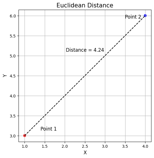 Euclidean Distance (Image generated by Author)
Used commonly for continuous data, it’s the straight-line distance between two points in Euclidean space. Euclidean Distance (Image by Author)
In this equation:
- xi and yi are the coordinates of points x and y in the i-th dimension, respectively.
- The term (xi−yi)² computes the squared difference between the coordinates of x and y in each dimension.
- The summation ∑ adds up these squared differences across all dimensions.
- The square root is applied to the sum of squared differences, yielding the final distance.
In the image, this would be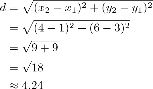 Manhattan Distance
 Manhattan Distance (Image by author)
Also known as the city block distance, it is the sum of the absolute differences of their Cartesian coordinates. Unlike the straight-line distance measured by Euclidean distance, Manhattan distance calculates the distance traveled along axes at right angles. It’s preferred for categorical data. Manhattan Distance (Image by Author)
- The term ∣xi−yi∣ calculates the absolute difference between the coordinates of x and y in each dimension.
- The summation ∑ aggregates these absolute differences across all dimensions.
Following the example above this would be: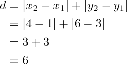 Minkowski Distance
It’s a generalization of both Euclidean and Manhattan distances. It introduces a parameter p that allows different distance metrics to be calculated. The Minkowski distance includes both the Euclidean distance and the Manhattan distance as special cases when p=2 and p=1, respectively.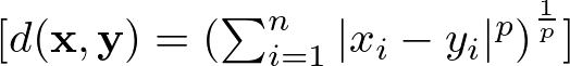 Minkowski Distance (Image by Author)
Here:
- ∣xi−yi∣ calculates the absolute difference between the coordinates of x and y in the i-th dimension.
- p is a positive integer that determines the order of the Minkowski distance. When p changes, the nature of the distance measurement changes as well.
- The summation ∑ aggregates these absolute differences, raised to the power of p, across all dimensions.
- Finally, the p-th root of the sum gives the Minkowski distance.
Step 2: Identify Nearest Neighbors
After calculating the distances, the algorithm sorts them and selects the ‘k’ smallest distances. This step identifies the ‘k’ nearest neighbors to the current data point.
Step 3: Aggregate Nearest Neighbors
For Classification KNN aggregates the class labels of the ‘k’ nearest neighbors to predict the class of the current data point. The most common class label among the ‘k’ nearest neighbors is chosen as the prediction. Aggregate Nearest Neighbors — Classification (Image by Author)
where Cq is the predicted class for the current data point, and Cni is the class of the ‘k’ nearest neighbors.
For Regression KNN calculates the mean (or sometimes median) of the target values of the ‘k’ nearest neighbors to predict the value for the current data point.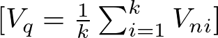 Aggregate Nearest Neighbors — Regression (Image by Author)
where Vq is the predicted value for the query instance, and Vni is the target value of the ‘k’ nearest neighbors.
Step 4: Predict the Outcome
Based on the aggregation in Step 3, KNN predicts the class (for classification tasks) or value (for regression tasks) of the query instance. This prediction is made without the need for an explicit model, as KNN uses the dataset itself and the distances calculated to make predictions.
2.2: Choosing the Right K Value
Choosing the right number of neighbors, or ‘k’, in the K-Nearest Neighbors (KNN) algorithm is so important, that could be considered as one of the algorithm's limitations, as a poor choice would likely lead to a poor performance. The perfect ‘k’ helps the model catch the real patterns in the data, while the wrong ‘k’ could lead to guesses that are off the mark. Fortunately, there are a few techniques we can use to better understand what ‘k’ to use.
Cross Validation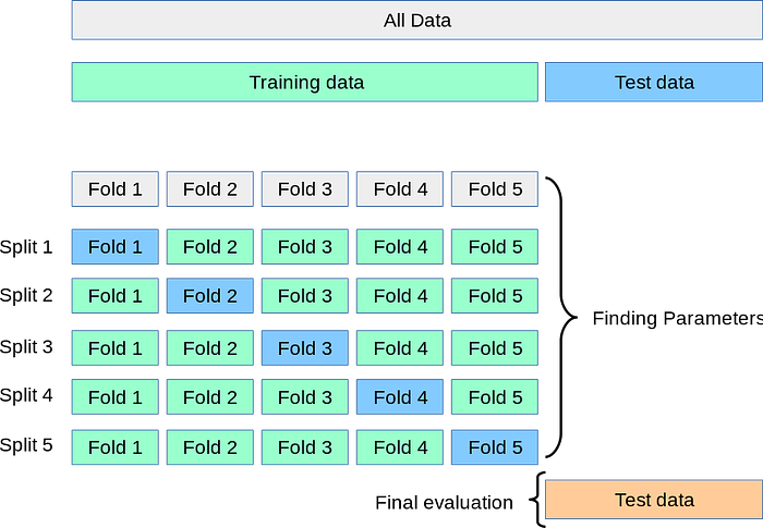 Image by sci-kit learn documentation
Think of this as trial runs. You divide your data into ‘k’ groups, for every run you use one group as a test and all the other ones to train the model. Using cross-validation avoids overfitting, and it’s likely to be a better representation of reality. Then, we test different k-values and pick the k which reports the best accuracy.
Error Rate Analysis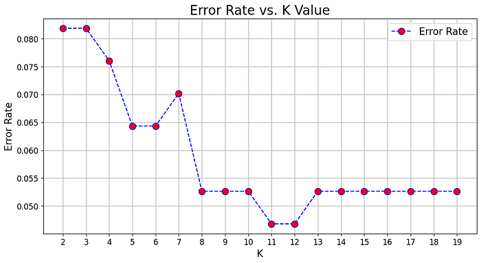 Error Rate Analysis (Image by author)
This is about drawing a graph of ‘how wrong your model gets’ against different ‘k’ values. You’re looking for the ‘k’ where things start to level off, showing you’re getting the most bang for your buck without the model’s performance going downhill. In the picture above 11 would be the best K to choose, as it gives the lowest error rate.
Knowing Your Field
This may sound obvious, but knowing what you’re studying can hint at the best ‘k’. If you know how your data tends to group or spread out, you can pick a ‘k’ that makes sense for the real-world scenario you’re trying to model.
2.3: How to choose the right Distance Metric
Choosing the right distance metric is also a critical step in optimizing the KNN for specific datasets and problem domains. Using an analogy, it’s like choosing the right glasses to see the data clearly: the better the fit, the clearer you’ll see your ‘k’ nearest neighbors and the better your predictions will be.
To understand what’s the best distance to use, you should ask yourself the following questions:Image by Author
1. What’s your data like?
Continuous vs. Categorical: If your data is all about numbers and measurements (continuous data), Euclidean distance is your go-to, because it measures straight lines between points. For data that’s more about categories (like types of fruit, where “apple” and “orange” aren’t on a scale), Hamming distance, which checks if features match, makes more sense.
Scale of Features: Look out for different scales in your dataset. If you don’t adjust for this, your distances could be thrown off, making some features louder than others. Normalize your data or switch to Manhattan distance, which isn’t as thrown off by different scales.
2. How big is your data?
When your dataset is really wide (lots of features), traditional ideas of closeness get wonky, and everything starts to seem far apart. Here, reducing dimensions or picking metrics suited for the big stage, like cosine similarity for text, can keep things in perspective.
3. How is your data spread out?
The way your data is distributed matters. If outliers are a big deal in your dataset, Manhattan distance might be your ally since it doesn’t get as shaken up by extreme values compared to Euclidean distance.
4. Need for speed?
Some distance metrics are computationally more intensive than others. Metrics like Manhattan distance can be computationally more efficient than Euclidean distance in certain implementations since it lacks the square root operation.
Lastly, don’t marry the first metric you meet. Play the field, try different metrics, and see which one makes your model the happiest through cross-validation.
3: KNN in Practice
3.1 KNN From Scratch in Python
Now let’s see what we described in math terms looks like in Python code. Let’s start by defining the whole class and then break it down into smaller pieces:
import numpy as np
from collections import Counter

class KNN:
    def __init__(self, k=3, distance_metric='euclidean'):
        self.k = k
        self.distance_metric = distance_metric

    def _euclidean_distance(self, x1, x2):
        """
        Compute the Euclidean distance between two vectors

        Parameters
        ----------
        x1 : array-like
            A vector in the feature space
        x2 : array-like
            A vector in the feature space

        Returns
        -------
        float
            The Euclidean distance between x1 and x2
        """
        return np.sqrt(np.sum((x1 - x2)**2))

    def _manhattan_distance(self, x1, x2):
        """
        Compute the Manhattan distance between two vectors

        Parameters
        ----------
        x1 : array-like
            A vector in the feature space
        x2 : array-like
            A vector in the feature space

        Returns
        -------
        float
            The Manhattan distance between x1 and x2
        """
        return np.sum(np.abs(x1 - x2))

    def _minkowski_distance(self, x1, x2):
        """
        Compute the Minkowski distance between two vectors

        Parameters
        ----------
        x1 : array-like
            A vector in the feature space
        x2 : array-like
            A vector in the feature space

        Returns
        -------
        float
            The Minkowski distance between x1 and x2
        """
        return np.sum(np.abs(x1 - x2)**self.k) ** (1/self.k)

    def fit(self, X, y):
        """
        Fit the model using X as training data and y as target values

        Parameters
        ----------
        X : array-like
            Training data
        y : array-like
            Target values
        """
        self.X_train = X
        self.y_train = y

    def predict(self, X):
        """
        Predict the class labels for the provided data

        Parameters
        ----------
        X : array-like
            Data to be used for prediction

        Returns
        -------
        array-like
            Predicted class labels
        """
        predicted_labels = [self._predict(x) for x in X]
        return np.array(predicted_labels)

    def _predict(self, x):
        """
        Predict the class label for a single sample

        Parameters
        ----------
        x : array-like
            A single sample

        Returns
        -------
        int
            The predicted class label
        """
        # Compute distances between x and all examples in the training set
        if self.distance_metric == 'euclidean':
            distances = [self._euclidean_distance(x, x_train) for x_train in self.X_train]
        elif self.distance_metric == 'manhattan':
            distances = [self._manhattan_distance(x, x_train) for x_train in self.X_train]
        elif self.distance_metric == 'minkowski':
            distances = [self._minkowski_distance(x, x_train) for x_train in self.X_train]
        else:
            raise ValueError("Invalid distance metric. Choose from 'euclidean', 'manhattan', 'minkowski'.")

        # Sort by distance and return indices of the first k neighbors
        k_indices = np.argsort(distances)[:self.k]
        # Extract the labels of the k nearest neighbor training samples
        k_nearest_labels = [self.y_train[i] for i in k_indices]
        # return the most common class label
        most_common = Counter(k_nearest_labels).most_common(1)
        return most_common[0][0]
Initialization
def __init__(self, k=3, distance_metric='euclidean'):
        self.k = k
        self.distance_metric = distance_metric
The KNN class first initializes two variables: k, and the distance metric. Here ‘k’, is the number of k-neighbors we want to use for the model, and the distance metric is a text field to specify what metric we want to use to compute the distance. In this example, we present three options — Euclidean, Manhattan, and Minkowski distance — but feel free to experiment with more distances.
Distance Methods
def _euclidean_distance(self, x1, x2):
        return np.sqrt(np.sum((x1 - x2)**2))

def _manhattan_distance(self, x1, x2):
        return np.sum(np.abs(x1 - x2))

def _minkowski_distance(self, x1, x2):
        return np.sum(np.abs(x1 - x2)**self.k) ** (1/self.k)
Next, we define three methods that will calculate the specified distance. They are just the Pythonic expression of the math formulas we defined before. Nothing fancy, and pretty straightforward.
Fit Method
def fit(self, X, y):
        self.X_train = X
        self.y_train = y
The fit method stores the X, and y, as class variables, which will later be called by the predict method.
_predict Method
def _predict(self, x):
        # Compute distances between x and all examples in the training set
        if self.distance_metric == 'euclidean':
            distances = [self._euclidean_distance(x, x_train) for x_train in self.X_train]
        elif self.distance_metric == 'manhattan':
            distances = [self._manhattan_distance(x, x_train) for x_train in self.X_train]
        elif self.distance_metric == 'minkowski':
            distances = [self._minkowski_distance(x, x_train) for x_train in self.X_train]
        else:
            raise ValueError("Invalid distance metric. Choose from 'euclidean', 'manhattan', 'minkowski'.")

        # Sort by distance and return indices of the first k neighbors
        k_indices = np.argsort(distances)[:self.k]
        # Extract the labels of the k nearest neighbor training samples
        k_nearest_labels = [self.y_train[i] for i in k_indices]
        # return the most common class label
        most_common = Counter(k_nearest_labels).most_common(1)
        return most_common[0][0]
This is the core method of the class. It first accesses the distance metric variable we initialized at the beginning of the class, then calculates the distances between the data point we want to predict and all the data points in the training set.
After calculating the distances, we sort them by ascending order and return the first k indices, where k is the number of neighbors we initialized at the beginning of the class.
Lastly, we retrieve the target values in the training dataset associated with the indices and return the most common value.
Note, that this last step would be different in case of regression, as would calculate the mean or median instead.
predict Method
def predict(self, X):
        predicted_labels = [self._predict(x) for x in X]
        return np.array(predicted_labels)
Finally, we define the predict method, which is a wrapper of the previous _predict method. What this method does is call the _predict method on all the observations in X, which are the observations we want to predict. Lastly, it returns all the predictions stored in a numpy array.
And, that’s it! Pretty cool, right? Very simple algorithm, but still very powerful.
For the full code, and a practical implementation look at this Jupyter Notebook:
models-from-scratch-python/K-Nearest Neighbors Classifier/demo.ipynb at main ·…
Repo where I recreate some popular machine learning models from scratch in Python …
github.com
3.2 Implementing KNN with Scikit-Learn
As I usually say in my articles, the code above is likely what you don’t want to use in production, as I created it just for educational purposes. Instead, we can take advantage of the great sci-kit learn library, which offers a better and more efficient version of the algorithm, and we just a few lines of code.
from sklearn import datasets
from sklearn.model_selection import train_test_split
from sklearn.preprocessing import StandardScaler
from sklearn.neighbors import KNeighborsClassifier
from sklearn.metrics import accuracy_score

# Load iris dataset
iris = datasets.load_iris()
X = iris.data
y = iris.target

# Split the data into training and test sets
X_train, X_test, y_train, y_test = train_test_split(X, y, test_size=0.2, random_state=42)

# Standardize the features
sc = StandardScaler()
X_train_std = sc.fit_transform(X_train)
X_test_std = sc.transform(X_test)

# Create KNN classifier
knn = KNeighborsClassifier(n_neighbors=3)

# Fit the classifier to the data
knn.fit(X_train_std, y_train)

# Predict the labels of the test set
y_pred = knn.predict(X_test_std)

# Print the accuracy of the classifier
print(f'Accuracy: {accuracy_score(y_test, y_pred):.2%}')
# Accuracy 100.00%
For this example, we are using the Iris dataset, and defining a KNN with 3 Neighbors, and distance method Minkowski with p=2, which is the default distance method for KNN in sci-kit learn. As we can see the code works similarly to what we built from scratch.
Now feel free to use this code, and play with it.
4: Advantages and Challenges
4.1 Benefits of Using KNN
The K-Nearest Neighbors (KNN) algorithm, despite its simplicity, offers several compelling advantages that make it a valuable tool for both classification and regression tasks in machine learning. Its intuitive approach, based on the principle that similar instances tend to be near each other, allows it to perform remarkably well across a wide range of applications. Here, we explore the key benefits of using KNN:
Simple and Intuitive
KNN wins big points for being straightforward. It’s the kind of algorithm that doesn’t need you to be a machine-learning wizard to use effectively. The whole concept of looking for the nearest neighbors based on how close they are is something anyone can understand. This makes this algorithm a friendly starting point for beginners.
No Assumptions About Data
Unlike many machine learning algorithms that make assumptions about the distribution of the data, KNN is non-parametric. This means it makes no prior assumptions about the form of the data, allowing it to be effective in scenarios where the data distribution is unknown or the relationship between variables is complex.
Adaptability
Adjustments to the number of neighbors (‘k’) or the choice of distance metric can significantly change the algorithm’s behavior, allowing for fine-tuning to specific datasets or problem characteristics. This adaptability extends to its capacity to deal with changes in the data, as KNN naturally incorporates new information during prediction without needing to be retrained.
Robustness to Noisy Data
In a perfect world, data would be clean and tidy. In the real world, not so much. KNN is pretty good at dealing with messy, noisy data. Since it looks at several neighbors to make a decision, a few oddballs here and there won’t throw it off track. Using a smart voting or averaging system can help make sure the reliable data gets more say.
4.2 Overcoming KNN Limitations
While K-Nearest Neighbors is a go-to for its straightforward approach and adaptability, it’s not without its flaws. Let’s walk through some of the main challenges you might bump into and talk about how to tackle them head-on.
Computational Complexity
The biggest gripe with KNN is how much it demands in terms of computation, especially with hefty datasets. It’s like trying to remember every person you’ve ever met — the more people, the harder it gets.
To overcome this, try to use efficient data structures such as KD-Trees or Ball Trees to reduce search time for nearest neighbors. Also, consider applying dimensionality reduction techniques like Principal Component Analysis (PCA) to trim down the excess features, making the distance calculation quicker and less of a headache.
For a comprehensive guide on PCA consider looking at this article:
Principal Component Analysis (PCA): From Scratch in Python
Eigen Decomposition, PCA Benefits & Pitfalls, and Python Code
medium.com
Sensitivity to Irrelevant Features
KNN treats every feature like it’s equally important, which isn’t always the case.
Here, two approaches you may follow are feature selection and scaling. Use feature selection to spotlight the features that matter, and scale your features so they all have an equal shot at influencing the outcome.
Handling of Categorical Data
KNN assumes numerical data for distance calculation, making the direct application to categorical data challenging.
Because of this, it’s important to encode categorical data using techniques like one-hot encoding before applying KNN. Also, use distance metrics specifically designed for categorical data, such as the Hamming distance.
Data Imbalance
In a dataset where one class overshadows the others, KNN might get a little biased towards the more common class.
In this case, we can trick KNN, and use one of its variants: weighted KNN, where the votes of the nearest neighbors are weighted by their distance, giving more influence to the closer neighbors.
Another approach would be applying sampling techniques to balance the dataset, such as oversampling the minority class or undersampling the majority class.
5: Beyond Basic KNN
5.1 Variants of KNN
The K-Nearest Neighbors algorithm, while powerful in its standard form, has inspired several variants designed to address its limitations and adapt to specific challenges. These variations extend KNN’s applicability and efficiency, making it even more versatile across a wider range of datasets and problem settings. Here, we explore some of the notable variants of the KNN algorithm.
Weighted KNN
This twist on KNN doesn’t treat all neighbors equally. Instead, it gives more say to the ones closer to the point you’re looking at. Think of it as paying more attention to your close friends’ opinions than acquaintances when making a decision. This can make your predictions sharper, especially when some neighbors should matter more than others.
Radius-Based KNN
Instead of counting neighbors, this version draws a circle (or sphere) of a fixed size around your point and considers anyone inside that space. It’s a bit like deciding who gets to come to your party based on how close they live. This is super handy for areas where your data points are all over the place in terms of how close together they are.
KD-Trees and Ball Trees
These are fancy ways of organizing your data so you can find your nearest neighbors without having to check every single point. Imagine organizing your bookshelf so you can instantly grab books from a certain genre without looking through every book. It’s a game-changer for working with big datasets where finding neighbors the old-fashioned way would take too long.
Locally Sensitive Hashing (LSH) for KNN
LSH is like a shortcut for finding neighbors by grouping similar items into buckets. It’s a bit like sorting people into groups based on their interests so you can quickly find someone to chat with. This method can speed things up a lot, especially with huge datasets, but it’s a bit of a trade-off because you might not get as precise results.
KNN with Feature Learning
Some KNN variations are all about getting smarter at figuring out which features (or characteristics) of your data are important. Using tools like autoencoders or deep metric learning, KNN can better see which data points are truly close together. It’s akin to learning to read between the lines to understand what brings people together.
KNN for Imbalanced Data
When your data is lopsided, with way more examples of one thing than another, these KNN versions tweak how they count votes or choose neighbors to make sure the underdog gets a fair shake. It’s like making sure everyone in a small town gets heard, not just the folks who talk the loudest.
6: Conclusion
The magic of KNN lies in how it uses the idea of “nearness” to make predictions, a concept as old as time but incredibly effective for everything from sorting photos to predicting stock trends. Its flexibility is on full display across different sectors like healthcare, finance, and cybersecurity, where it’s not just about tagging data points but solving complex problems that matter.
We’ve also seen the different flavors of KNN that can be customized for specific challenges, whether it’s dealing with vast amounts of data or making sure smaller voices aren’t drowned out in imbalanced datasets. This adaptability is what makes KNN such a valuable tool in the toolbox of machine learning.
Of course, KNN isn’t perfect. It can be a bit of a resource hog, requires a bit of tuning to get ‘k’ and the distance metric just right, and doesn’t always play nice with irrelevant features or data of varying scales. But the good news is, that we’ve got strategies to tackle these issues, from smart data prep to using clever data structures, paving the way to make the most of what KNN has to offer.
Bibliography
- Altman, N. S. (1992). An introduction to kernel and nearest-neighbor nonparametric regression. The American Statistician, 46(3), 175–185. https://doi.org/10.1080/00031305.1992.10475879
- Cover, T., & Hart, P. (1967). Nearest neighbor pattern classification. IEEE Transactions on Information Theory, 13(1), 21–27. https://doi.org/10.1109/TIT.1967.1053964
- Fix, E., & Hodges, J. L. (1951). Discriminatory analysis, nonparametric discrimination: Consistency properties. USA Air Force School of Aviation Medicine, Randolph Field, Texas. Report Number 4.
- Guo, G., Wang, H., Bell, D., Bi, Y., & Greer, K. (2003). KNN model-based approach in classification. OTM Confederated International Conferences” On the Move to Meaningful Internet Systems”, 986–996. https://doi.org/10.1007/978-3-540-39964-3_62
You made it to the end. Congrats! I hope you enjoyed this article, if so consider leaving a like and following me, as I will regularly post similar articles. My goal is to recreate all the most popular algorithms from scratch and make machine learning accessible to everyone.